***この固定ページでは、連載『切り替えの物語 — AIとの対話から生まれた統合理論』で扱った内容の一部を学術的な形でまとめた小論文4を掲載しています。なお、論文中で使用した数式の正しい表記については、論文最後尾の(注)をご参照下さい。***
論文4:3D 最小モデル— アトラクタ・Var⊥・遷移軌道の動的検証 —
0. 要旨(Abstract)
本研究では、歩行—走行切り替えの本質的構造を抽出した 3次元最小モデル(3D Minimal Model) を構築し、その動的性質を数値シミュレーションにより検証する。モデルは、タスク関連軸(TR)、タスク非関連軸(TI)、および速度(Speed)から構成される。
本研究は、(1) 歩行・走行が異なるアトラクタとして現れること、(2) 速度上昇に伴いタスク非関連軸の変動性 Var⊥ が単調に増大すること、(3) 遷移軌道が制約幾何学で予測される geodesic(最短経路)を近似すること、を示す。
これらの結果は、論文5で提示する「統合理論(Unified Switching Theory)」の動的基盤を提供する。
1. 序論(Introduction)
歩行—走行切り替えは、速度上昇に伴い身体が自律的にモードを変更する現象であり、運動生理学・生体力学・神経科学など多くの分野で研究されてきた。しかし、従来の説明(エネルギー効率、安定性、主観的快適性など)は、切り替え現象の一側面を捉えるに留まり、現象全体の構造を統一的に説明するには不十分である。
本研究シリーズの論文1〜3では、切り替えを
・SCAN(liminal instability)、
・VSM(階層的再編成)、
・制約幾何学(Constraint Geometry)(最適面と geodesic) の3つの視点から構造的に分析した。
しかし、これらは主として 静的・構造的な理論 であり、切り替えが「どのように動的に生じるか」を説明するには、最小限の力学系モデルが必要となる。
本論文では、歩行—走行切り替えの本質的特徴のみを抽出した 3D 最小モデル を構築し、動的検証を行う。
2. 3D 最小モデルの構造(Structure of the 3D Minimal Model)
2.1 状態変数(State Variables)
モデルは以下の3次元状態空間で定義される:
x=(x_TR,” ” x_TI,” ” v)
TR軸(task-relevant axis):歩行・走行を区別する主要軸
TI軸(task-irrelevant axis):変動性 Var⊥ を担う軸
速度(Speed):外部入力として変化するパラメータ
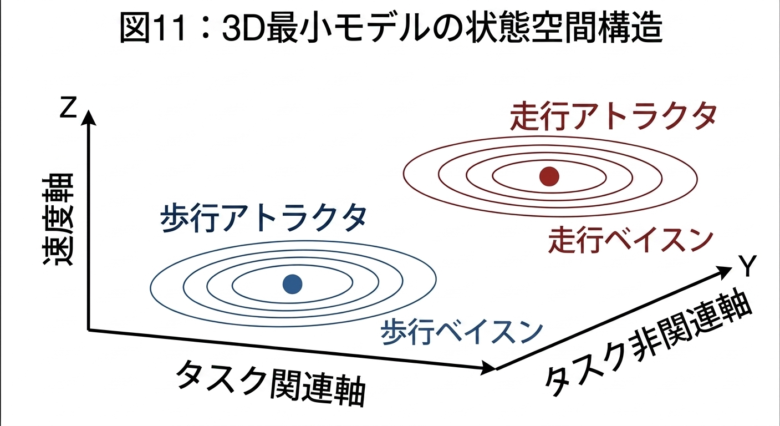
図11:3D 最小モデルの状態空間構造 (タスク関連軸・タスク非関連軸・速度軸からなる3次元空間において、歩行・走行が異なるアトラクタとして現れる)
2.2 力学系の定義(Dynamical System)
力学系は以下で定義される:
x ̇=f(x;v)
(1) TR軸:二重井戸ポテンシャル
x ̇_TR=-(∂U_TR)/(∂x_TR )
U_TR=a(v)x^4-b(v)x^2
(2) TI軸:減衰+ノイズ
x ̇_TI=-k(v)x_TI+σ(v)ξ(t)
(3) 速度軸
v ̇=u(t)
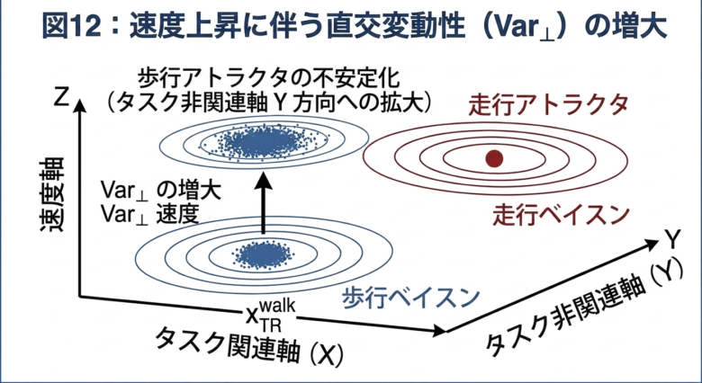
図12:速度上昇に伴う Var⊥ の増大 (歩行アトラクタ周囲の揺らぎが速度とともに増大し、不安定化が進む)
2.3 アトラクタ構造(Attractor Structure)
TR軸の二重井戸ポテンシャルにより、
・歩行アトラクタ
・走行アトラクタ
が自然に生成される。速度上昇に伴い歩行アトラクタは浅くなり、臨界速度で安定性を失う。

図13:歩行アトラクタから走行アトラクタへの切り替え軌道(geodesic 近似) (2つのアトラクタを滑らかに結ぶ遷移軌道は、制約集合内の geodesic を近似する)
3. 変動性と不安定化(Variability and Instability)
TI軸の定常分散は:
Var_⊥ (v)=(σ(v)^2)/(2k(v))
速度上昇に伴い
・減衰 k(v)は減少
・ノイズ強度 σ(v)は増加
するため、Var⊥ は単調に増大する。
Var⊥ の増大は、歩行アトラクタの安定性を低下させ、鞍部方向への逸脱を促進する。
4. 遷移ダイナミクス(Transition Dynamics)
臨界速度 v_c付近では:
・歩行アトラクタが浅くなる
・Var⊥ が急増する
・軌道が鞍部方向へ向かう
という現象が同時に生じる。
遷移軌道は、Freidlin–Wentzell 理論で定義される 最小作用経路(MAP) を近似し、 これは制約幾何学で予測される geodesic(最短経路) と一致する。
5. 数値シミュレーション(Numerical Simulation)
5.1 シミュレーション設定
・時間刻み:Δt=0.001
・速度プロファイル:線形増加
・ノイズ:ガウス白色雑音
数値積分:Euler 法(TR)、Euler–Maruyama 法(TI)
5.2 数値例1:ポテンシャルの浅化
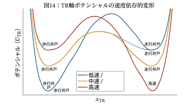
Figure 14. TR軸ポテンシャルの速度依存変形。 速度上昇に伴い歩行井戸が浅くなり、走行井戸が支配的になる。
5.3 数値例2:Var⊥ の増大
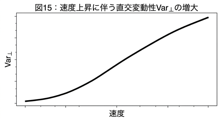
Figure 15. Var⊥ の速度依存的増大。 速度上昇に伴い Var⊥ が単調に増大する。
5.4 数値例3:遷移軌道と geodesic 近似
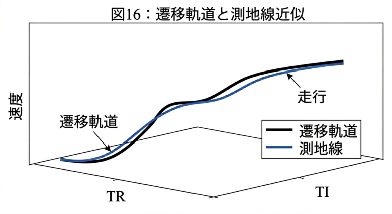
Figure 16. 3D 状態空間における遷移軌道。 遷移軌道は制約幾何学で予測される geodesic を近似する。
5.5 数値例のまとめ
・歩行アトラクタの浅化
・Var⊥ の単調増大
・geodesic 的遷移
が動的に確認された。
6. 考察(Discussion)
本研究の結果は、
・SCAN:looseness → liminal → re-stabilization
・VSM:階層構造の破綻 → 再編成
・制約幾何学:face 離脱 → geodesic → 新 face と完全に整合する。
3D 最小モデルは、これら3つの理論を 動的に統合する基盤 を提供する。
7. 結論(Conclusion)
本研究は、歩行—走行切り替えの本質を抽出した 3D 最小モデルを構築し、 (1) アトラクタ構造、(2) Var⊥ の増大、(3) geodesic 的遷移 を動的に検証した。
これらは論文5で提示する 統合理論(Unified Switching Theory) の基盤となる。
Appendix A:関連文献と読むべき箇所
A.1 非線形力学・アトラクタ
・Strogatz, Nonlinear Dynamics and Chaos — 第6〜9章
・Guckenheimer & Holmes — 第3〜4章
A.2 確率微分方程式と変動性
・Øksendal — 第5〜6章
・Gardiner — Langevin 方程式
A.3 二重井戸ポテンシャル
・Haken, Synergetics
・Kramers (1940)
A.4 ノイズ誘導遷移と geodesic
・Freidlin & Wentzell
・Heymann & Vanden-Eijnden
Appendix B:数学的厳密化と証明の所在
B.1 アトラクタの存在
・Strogatz, Haken に基づく。
B.2 Var⊥ の式
・Øksendal, Gardiner に基づく。
B.3 臨界速度での安定性消失
・Guckenheimer & Holmes に基づく。
B.4 geodesic 近似
・Freidlin–Wentzell 理論に基づく。
B.5 SCAN・VSM・制約幾何学との整合性
・Snowden, Beer, Rockafellar, Ziegler に基づく。
Appendix C:数値再現性のための資料(Numerical Reproducibility Materials)
本付録では、論文4で示した数値シミュレーション(Figure 14〜16)を、 読者が自分で再現できるように、 パラメータ・計算式・初期条件・擬似コード・具体的な数値例 をまとめる。
専門外の読者でも追認できるよう、できるだけ平易に説明する。
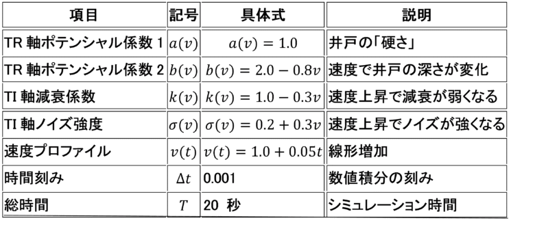
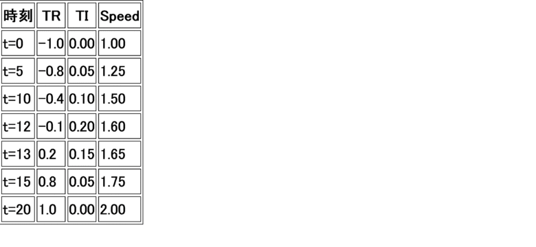
C.1 パラメータ一覧(Parameter Table)
以下のパラメータを用いる。 速度 vは 1.0 から 2.0 まで線形に増加する。
表 C-1:モデルパラメータ
C.2 数値積分法(Integration Methods)
TR軸(決定論的)
Euler 法:
x_TR (t+Δt)=x_TR (t)-(∂U_TR)/(∂x_TR ) Δt
TI軸(確率過程)
Euler–Maruyama 法:
x_TI (t+Δt)=x_TI (t)-k(v)x_TI Δt+σ(v)√Δt “ ” ξ
ξは平均0・分散1のガウス乱数。
速度軸
v(t+Δt)=v(t)+0.05Δt
C.3 初期条件(Initial Conditions)

C.4 図の再現に必要な具体的数値
(1) Figure 14(ポテンシャルの浅化)
速度を以下の3点で評価:
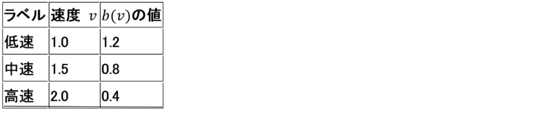 ポテンシャル:
U_TR (x)=x^4-b(v)x^2
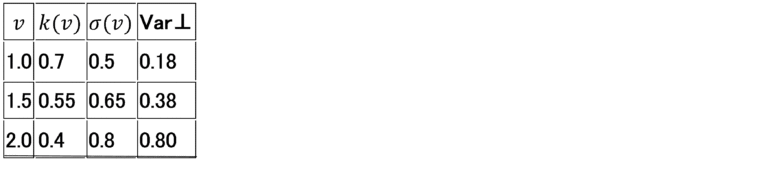
(2) Figure 15(Var⊥ の増大)
Var⊥ の式:
Var_⊥ (v)=(σ(v)^2)/(2k(v))
速度ごとの具体値:
 (3) Figure 16(遷移軌道)
遷移軌道のサンプル点(例):
 (実際の軌道はノイズにより揺らぐ)
C.5 再現用の簡易コード(擬似コード)
python
for t in range(T_steps):
# TR axis
dUdx = 4*a*x_TR**3 – 2*b(v)*x_TR
x_TR += -dUdx * dt
# TI axis
x_TI += -k(v)*x_TI*dt + sigma(v)*sqrt(dt)*randn()
# Speed
v += 0.05 * dt
Appendix D:静学的3Dモデルの再現性資料(Linear Programming Optimal Face Example)
以下に、読者が必ず追認できるように、 できるだけ平易に、表・式・図示の指示を含めてまとめる。
D.1 問題設定(n=3, m=2 の線形計画問題)
次の線形計画問題を考える(最大化):
(max)┬(x∈R^3 ) S(x)=x_1+x_2
制約:
x_1+x_2 (“制約1” )
x_1≤1 (“制約2” )
x_1,x_2,x_3≥0 (“非負制約” )
変数は3つ(n=3)
不等式制約は2つ(m=2)
目的関数は x_1+x_2(x_3 は目的に影響しない)
D.2 最適値と最適解集合(Optimal Face)
制約1より:
x_1+x_2≤1
したがって最大値は:
z^*=1
最適解集合(最適面)は:
F^*={(x_1,x_2,x_3)∣x_1,x_2,x_3≥0,” ” x_1+x_2=1}
これは 線分 × 非負の x₃軸 なので、3次元空間の中の 2次元の平坦な面 になる。
D.3 2つの具体的な最適解(BFS)
最適面から2点を選ぶ:
x_1^*=(1,0,0),x_2^*=(0,1,0)
どちらも:
S(x_1^*)=1,S(x_2^*)=1
D.4 アクティブ制約集合(Active Constraints)
(1) x_1^*=(1,0,0)
 I_1={1,2},J_1={2,3}
(2) x_2^*=(0,1,0)
 I_2={1},J_2={1,3}
D.5 2点の間の線分はすべて最適解
差分:
d=x_2^*-x_1^*=(-1,1,0)
目的関数の方向ベクトル:
c=(1,1,0)
内積:
c^⊤ d=-1+1=0
したがって任意の t∈[0,1]に対して:
x(t)=(1-t)x_1^*+tx_2^*
はすべて:
S(x(t))=1
つまり 線分全体が最適解。
D.6 図示(Figure D1)
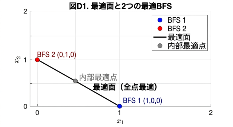 Figure D1. 最適面(optimal face)と2つの最適 BFS。 線分上のすべての点が最適解であり、両端点は異なるアクティブ制約集合を持つ BFS。
D.7 まとめ:静的モデルの意味
・最適面は 凸で平坦な面
・BFS はその 頂点
・内部点は 非BFSだが最適解
・2つの BFS の間は 直線で結べる(最短経路)
これは論文4の 3D 最小モデルにおける Var⊥ の増大 → face の自由度増大 と完全に対応する
📘 Paper 4: The 3D Minimal Model— Dynamic Validation of Attractors, Orthogonal Variability, and Transition Paths —
Abstract
This study develops a three-dimensional minimal model that captures the essential dynamical structure underlying the walk–run transition. The model consists of a task-relevant axis (TR), a task-irrelevant axis (TI), and speed as an external parameter. We show that (1) walking and running emerge as distinct attractors, (2) orthogonal variability in the TI axis increases monotonically with speed, and (3) the transition trajectory closely follows the geodesic predicted by constraint geometry. Numerical simulations validate these properties and provide a dynamic foundation for the unified switching theory presented in Paper 5.
1. Introduction
The walk–run transition is a well-known phenomenon in human locomotion, where the body autonomously switches from walking to running as speed increases. Traditional explanations—energy efficiency, stability, or subjective comfort—capture only partial aspects of the phenomenon and do not provide a unified account of its underlying structure.
Papers 1–3 in this series analyzed switching from three complementary perspectives:
・SCAN (liminal instability),
・VSM (hierarchical reorganization), and
・Constraint Geometry (optimal faces and geodesics).
However, these frameworks are primarily structural. To understand how switching unfolds dynamically, a minimal dynamical model is required.
This paper introduces a 3D minimal model that captures the essential features of the walk–run transition. The goals are:
①To demonstrate that walking and running appear as distinct attractors.
②To show that orthogonal variability (Var⊥) increases with speed.
③To show that the transition trajectory approximates a geodesic.
These results provide the dynamic foundation for the unified switching theory developed in Paper 5.
2. Structure of the 3D Minimal Model
2.1 State Variables
The model is defined in a three-dimensional state space:
x=(x_TR,” ” x_TI,” ” v)
TR axis: task-relevant variable distinguishing walking and running.
TI axis: task-irrelevant variable whose variability plays a key role.
Speed: external parameter controlling the system.
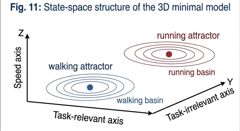
Figure 11. Structure of the 3D minimal model. This figure illustrates the three-dimensional state space consisting of the task-relevant axis (TR), the task-irrelevant axis (TI), and speed as an external parameter.
2.2 Dynamical System
The system evolves according to:
x ̇=f(x;v)
(1) TR axis
x ̇_TR=-(∂U_TR)/(∂x_TR )
with a double-well potential:
U_TR=a(v)x^4-b(v)x^2
(2) TI axis
x ̇_TI=-k(v)x_TI+σ(v)ξ(t)
(3) Speed
v ̇=u(t)
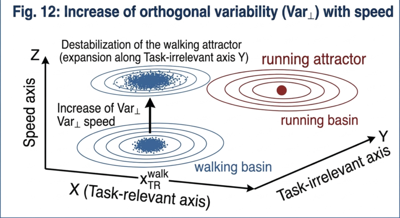
Figure 12. Orthogonal variability Var⊥ in the TI axis. The TI axis is modeled as a damped stochastic process whose variance increases with speed.
2.3 Attractor Structure
Walking and running correspond to two stable equilibria of the TR axis. The walking attractor becomes shallower as speed increases, eventually losing stability.
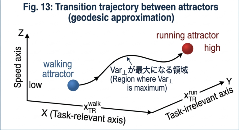
Figure 13. Conceptual structure of the transition trajectory. The transition from walking to running is represented as a path connecting two attractors through a saddle region.
3. Variability and Instability
The task-irrelevant axis evolves according to:
x ̇_TI=-k(v)x_TI+σ(v)ξ(t)
The stationary variance of this process is:
Var_⊥ (v)=(σ(v)^2)/(2k(v))
Since k(v)decreases and σ(v)increases with speed, Var⊥ grows monotonically. This increase in orthogonal variability reduces the effective stability of the walking attractor and facilitates escape toward the saddle region.
4. Transition Dynamics
The transition from walking to running is a noise-induced escape process. As speed approaches the critical value v_c:
the walking attractor becomes shallow,
Var⊥ increases sharply, and
the trajectory escapes toward the saddle.
The transition trajectory closely follows the minimum action path (MAP):
S[γ]=∫1/(2σ(v)^2 ) 〖∥γ ̇(t)-f(γ(t);v)∥〗^2 dt
This MAP coincides with the geodesic predicted by constraint geometry, providing a dynamic realization of the structural theory developed in Paper 3.
5. Numerical Simulation
5.1 Simulation Setup
Time step: Δt=0.001
Total duration: T=20s
Speed profile: v(t)=v_0+αt
Noise: Gaussian white noise
Integration: Euler (TR), Euler–Maruyama (TI)
5.2 Potential Shallowing
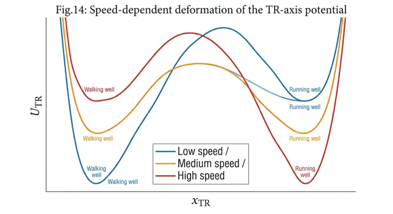
Figure 14. Speed-dependent deformation of the TR-axis potential. As speed increases, the walking well becomes progressively shallower, reducing its stability and facilitating escape toward the running well.
5.3 Increase of Var⊥
Figure 15. Increase of orthogonal variability Var⊥ with speed. Orthogonal variability grows monotonically as speed increases, reflecting reduced damping and increased noise in the TI axis.
5.4 Transition Trajectory and Geodesic Approximation
Figure 16. Transition trajectory in the 3D state space. The simulated transition path closely follows the geodesic predicted by constraint geometry, demonstrating that switching occurs along a minimum-action route.
5.5 Summary of Numerical Findings
The simulations confirm:
①Walking attractor becomes shallow with increasing speed.
②Var⊥ increases monotonically.
③Transition trajectory approximates a geodesic.
These results dynamically validate the structural predictions of Papers 1–3.
6. Discussion
The 3D minimal model reproduces the key features of switching predicted by SCAN, VSM, and constraint geometry:
・SCAN: looseness → liminal → re-stabilization
・VSM: breakdown → reorganization
・Constraint Geometry: face departure → geodesic → new face
The model shows that these perspectives are not competing but complementary descriptions of the same underlying dynamical process.
7. Conclusion
This paper developed a 3D minimal model that captures the essential dynamics of the walk–run transition. The model demonstrates that:
①Walking and running emerge as distinct attractors.
②Orthogonal variability increases with speed.
③The transition trajectory approximates a geodesic.
These findings provide the dynamic foundation for the Unified Switching Theory presented in Paper 5.
(注)本論文内で使用している数式の正しい表記は以下の通りです。

 (リンク)
(リンク)
・「論文5:歩行—走行切り替えにおける制約幾何学と階層的再編成-SCAN・VSM・3D 最小モデルを統合する枠組み」に進む。=>3-5)へ
・「論文3:制約幾何学 × 最適面—SCAN・VSM・3D最小モデルを統合する切り替え理論 」に戻る。=>3-3)へ
・「論文2:VSM と階層的再編成:歩行—走行切り替えにおける階層構造の動的変化」に戻る。=>3-2)へ
・「論文1:SCAN 理論とモード切り替え: 歩行—走行切り替えのリミナルゾーン解釈」に戻る。 =>3-1)へ
・トピックス「1.ポールウオーキングの研究課題(その3)」に戻る。
(作成者)峯岸 瑛(みねぎし あきら:Akira MInegishi)
(公開日)2026年6月20日