Appendix (A–D):
Supplementary Materials for the Unified Theory of Stability, Variability, and Switching
Overview
This appendix provides the mathematical foundations, parameter definitions, visual diagrams, and conceptual framework that support the unified theory presented in Paper A. The materials are organized to guide the reader from formal derivations, through model parameters, to visual intuition, and finally to the SCAN framework, which integrates somatic, cognitive, and action-level processes.
*****
Navigation
Structure of the Appendix
Appendix A — Mathematical Foundations and Proofs
Formal derivations of the key results used throughout Paper A, including:
・Stability as potential curvature
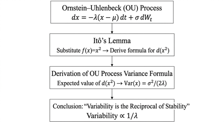
・Variability as the inverse of stability (OU process + Itô’s lemma)
・Existence of the liminal zone
・Noise-driven switching probability
・Intuitive explanation of Itô’s lemma
・How OU dynamics and Itô’s lemma jointly produce the variability formula
This appendix establishes the mathematical backbone of the theory.
→ Proceed to Appendix A
Appendix B — Parameter Definitions
A complete list of all variables, parameters, and initial conditions used in the models and simulations:
・State variables
・Dynamical parameters
・Noise and variability parameters
・Summary tables for reproducibility
This appendix ensures transparency and allows readers to replicate the results.
→ Proceed to Appendix B
Appendix C — Additional Diagrams
Visual supplements that reinforce the mathematical results:
・Figure C1: Stability landscape (Walking–Liminal–Running)
・Figure C2: Variability curve (inverse of stability)
・Figure C3: Switching probability vs variability
→ Proceed to Appendix C
Appendix D — SCAN Formalization
A formal description of the Somatic–Cognitive–Action Network (SCAN), which provides the behavioral and physiological interpretation of the mathematical model:
・Definitions of S, C, and A
・SCAN’s role in monitoring stability and variability
・SCAN’s involvement in switching
・Formal dynamical representation
・SCAN behavior in the liminal zone
・Figure D1: SCAN Loop Diagram
This appendix integrates the stochastic model with human motor control.
→ Proceed to Appendix D
How to Use This Appendix
Readers may approach the appendix in two ways:
1. Mathematical-first pathway
A → B → C → D
・For readers interested in formal derivations and reproducibility.
2. Conceptual-first pathway
D → C → A → B
・For readers who prefer to understand the behavioral framework first.
Both pathways lead to the same unified understanding of stability, variability, and switching.
Summary
The appendices collectively provide:
・A rigorous mathematical foundation (Appendix A)
・Complete parameter transparency (Appendix B)
・Clear visual intuition (Appendix C)
・A unifying behavioral framework (Appendix D)
Together, they form a coherent and comprehensive supplement to Paper A.
******
Appendix A. Mathematical Foundations and Proofs
~Formal Derivations and Intuitive Explanations for Stability, Variability, the Liminal Zone, and Switching Dynamics~
This appendix presents the mathematical foundations underlying the unified theory of switching and variability in human locomotion. The goal is not to provide exhaustive, formal proofs in the style of pure mathematics, but to offer clear, rigorous derivations that support the theoretical claims made in Paper A. To aid readers who may be new to stochastic processes, we also include intuitive explanations of key concepts such as the Ornstein–Uhlenbeck (OU) process and Itô’s lemma.
The appendix is organized as follows:
①A.1 Stability as Potential Curvature
②A.2 Variability as the Inverse of Stability (via the OU process)
③A.3 Existence of a Liminal Zone (Saddle Region)
④A.4 Why Increased Variability Raises Switching Probability
⑤A.5 An Intuitive Explanation of Itô’s Lemma
⑥A.6 How the OU Process and Itô’s Lemma Work Together
A.1 Stability as Potential Curvature
Locomotor states (e.g., walking, running) are modeled as points x∈Revolving in a potential landscape V(x). Stable locomotor modes correspond to local minima of the potential.

A.2 Variability as the Inverse of Stability (via the OU Process)
 A.3 Existence of a Liminal Zone (Saddle Region)
If the potential has two stable minima (walking and running), a shallow region must exist between them.
 A.4 Why Increased Variability Raises Switching Probability
Switching occurs when noise-driven fluctuations push the system over the saddle.
 A.5 An Intuitive Explanation of Itô’s Lemma (For Beginners)
Itô’s lemma can be understood as:
“The chain rule for a world with noise.”
 This correction is precisely what allows us to derive the variance of the OU process.
A.6 How the OU Process and Itô’s Lemma Work Together
The OU process provides a model of stability with noise, and Itô’s lemma provides the mathematical machinery to analyze it.
Their relationship can be summarized as:
 Thus:
Thus:
The combination of the OU process and Itô’s lemma yields the core result of Paper A: “Variability is the inverse of stability.”
Summary of Appendix A
This appendix established the following key results:
①Stability is quantified by potential curvature.
②Variability is the inverse of stability, derived using the OU process and Itô’s lemma.
③A liminal zone necessarily exists between walking and running attractors.
④Increased variability raises switching probability via noise-driven barrier crossing.
⑤Itô’s lemma provides the correct chain rule for noisy systems.
⑥The OU process + Itô’s lemma form the mathematical backbone of the unified theory.
******
Appendix B. Parameter Definitions
~Model Parameters, Initial Conditions, and Their Interpretations~
This appendix provides a complete list of the parameters, variables, and initial conditions used in the mathematical and simulation models presented in Paper A. The goal is to ensure transparency and reproducibility for readers who wish to replicate or extend the results.
Parameters are grouped into three categories:
①State Variables
②Dynamical Parameters
③Noise and Variability Parameters
A summary table is provided at the end of each subsection.
B.1 State Variables
The locomotor system is modeled using a low-dimensional state representation. The primary state variable is the locomotor mode coordinate x(t), which evolves within a potential landscape representing walking, the liminal zone, and running.
 These initial conditions correspond to the simulations shown in the main text and Appendix C.
B.2 Dynamical Parameters
The evolution of the locomotor state is governed by a potential function V(x)and its associated stability properties.
 These parameters appear in the linearization and stability proofs in Appendix A.
B.3 Noise and Variability Parameters
 This relationship is central to the unified theory of switching.
B.4 Summary Table (All Parameters)
 B.5 Notes on Reproducibility
・All simulations in Paper A and Appendix C use the parameter sets listed above.
・The OU-based variability model is consistent with the mathematical proofs in Appendix A.
・The potential landscape parameters (λ_W,λ_R,λ_L) correspond directly to the shapes shown in Figures A1–A4.
*****
Appendix C. Additional Diagrams
~Visual Supplements for Stability, Variability, and Switching Dynamics~
This appendix provides additional diagrams that visually support the mathematical results presented in Appendix A and the parameter definitions in Appendix B. The figures included here are designed to help readers intuitively understand the structure of the stability landscape, the relationship between stability and variability, and the mechanism by which variability increases switching probability.
C.1 Stability Landscape (Walking – Liminal – Running)
Figure C1. Stability Landscape Diagram
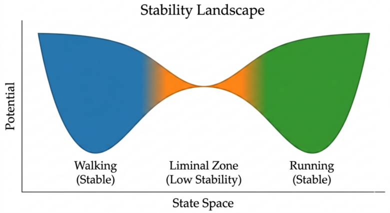 This diagram illustrates the potential landscape used throughout Paper A. It shows two stable attractor basins (walking and running) separated by a shallow saddle region (the liminal zone).
This figure visually supports:
・Appendix A.1
・Appendix A.3
・Appendix B
C.2 Variability Curve (Inverse of Stability)
Figure C2. Variability as the Inverse of Stability
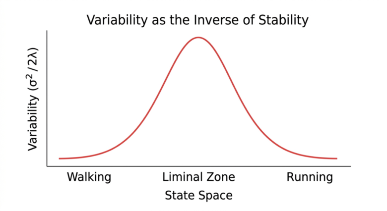
 This figure supports Appendix A.2 and A.6.
C.3 Switching Probability vs Variability
Figure C3. Switching Probability Increases with Variability
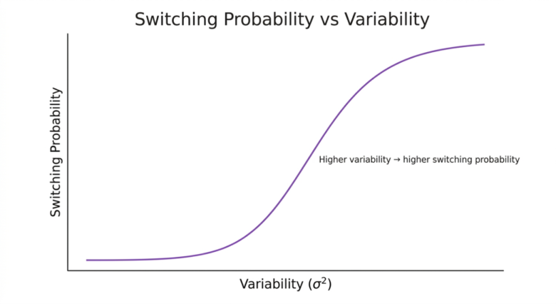
 This figure supports Appendix A.4.
Appendix C Summary
Appendix C provides three visual supplements:
 Together, these diagrams visually reinforce the mathematical results of Appendix A and the parameter definitions of Appendix B.
*****
Appendix D. SCAN Formalization
~A Formal Description of the Somatic–Cognitive–Action Network and Its Role in Switching and Variability~
This appendix provides a formal description of the Somatic–Cognitive–Action Network (SCAN), a three component framework used throughout Paper A to explain how humans regulate stability, variability, and switching during locomotion. SCAN serves as the conceptual bridge between the mathematical model (Appendix A) and the behavioral phenomena observed in human gait.
D.1 Overview of the SCAN Framework
SCAN consists of three interacting components:
・Somatic system (S) — bodily and physiological regulation
・Cognitive system (C) — attention, prediction, and evaluation
・Action system (A) — motor execution and control
These components form a closed-loop network:
S⟷C⟷A⟷S
The network continuously updates internal estimates of stability, variability, and environmental demands, enabling adaptive switching between locomotor modes.
D.2 Component Definitions
(1) Somatic System S
Represents physiological and biomechanical states:
・posture
・muscle tone
・joint stiffness
・energetic cost
・sensory feedback (vestibular, proprioceptive)
Formally, we denote the somatic state as:
S(t)∈R^n.
(2) Cognitive System C
Represents higher-level processes:
・prediction of future states
・evaluation of stability
・attention allocation
・decision thresholds for switching
Formally:
C(t)∈R^m.
(3) Action System A
Represents motor commands and control policies:
・step timing
・foot placement
・push-off force
・gait pattern selection
Formally:
A(t)∈R^k.
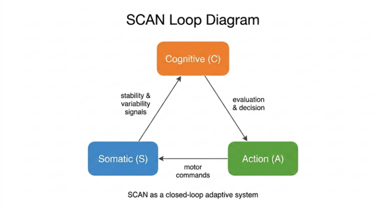 Figure D1 shows the SCAN framework as a closed-loop adaptive system. The Somatic system detects bodily fluctuations and stability changes. The Cognitive system evaluates these signals and determines whether a mode adjustment or switching is required. The Action system executes motor commands that influence the somatic state, completing the loop.
This continuous cycle allows SCAN to:
・monitor stability and variability in real time
・detect entry into the liminal zone
・increase switching readiness when variability rises
・coordinate transitions between walking and running
Thus, SCAN provides the behavioral and physiological interpretation of the stochastic dynamics formalized in Appendix A.
D.3 SCAN and Locomotor Mode Switching
SCAN regulates switching through continuous monitoring of stability and variability.
・The Somatic system detects increased variability (e.g., COM sway).
・The Cognitive system evaluates whether the current mode remains optimal.
・The Action system adjusts gait parameters or initiates a mode transition.
Switching occurs when:
C(t)” determines that ” λ(t)” is too low or ” Var(x)” too high”.
This aligns with the mathematical results in Appendix A.
D.4 Interaction Between Variability and SCAN
Variability plays two roles:
①As a signal — indicating reduced stability
②As a driver — enabling transitions across the liminal zone
SCAN interprets variability through the loop:
S(t)→C(t)→A(t).
Examples:
・Increased somatic noise → detected by S
・C interprets it as reduced stability
・A modifies gait or triggers switching
Thus, SCAN acts as the controller that interprets the stochastic dynamics described in Appendix A.
D.5 Formal Representation of SCAN
 D.6 SCAN and the Liminal Zone
The liminal zone corresponds to:
・low stability (λ≈0)
・high variability
・high cognitive involvement
SCAN behaves differently in this region:
・S detects instability
・C increases monitoring and prediction
・A becomes more exploratory (higher variability in motor commands)
 Summary of Appendix D
This appendix formalized the SCAN framework and its connection to the mathematical model:
①SCAN consists of Somatic, Cognitive, and Action components.
②These components form a closed-loop adaptive system.
③SCAN monitors stability and variability to regulate switching.
④Variability is both a signal and a driver of transitions.
⑤SCAN interacts with the potential landscape V(x)through its internal dynamics.
⑥The liminal zone is where SCAN becomes maximally engaged.
Together, SCAN and the stochastic model in Appendix A form a unified explanation of human locomotor switching.
*** Link ***
→ Paper A
→ Paper B
→ TOPICS – Key Themes and Research Directions in SPW —
→ English Article Series 1
→ English Gateway Page